02 — V: the vision model (a convolutional VAE)
What it is for, how it was trained, what it actually learned, and what that means for everything downstream.
1. The job of V in one sentence
V turns a 64×64×3 image (12,288 numbers) into a short vector z (16 numbers)
from which the image can be redrawn. Everything after V — the dynamics model,
the controller — never sees pixels again. They live entirely in z.
So the question V has to answer is: which 16 numbers summarise this frame? For our game the honest answer has three parts: where is the ball (x, y) and where is the paddle (x). Three numbers. We give the model 16 on purpose and watch how many it chooses to use.
Ha & Schmidhuber’s paper uses exactly this split. V is trained alone, on shuffled single frames, with no idea that time exists. That is a design decision, not a limitation: it means anything V learns is about the appearance of a frame, and anything about motion must be learned later by M. Keeping the two separate is what lets us ask, later, “where does velocity live?” and get a clean answer.
2. What a VAE is (the two-minute version)
A plain autoencoder is encoder(x) -> z -> decoder(z) -> x̂, trained to make
x̂ ≈ x. A variational autoencoder changes two things:
- The encoder outputs a distribution over
z, not a point: a meanμand a log-variancelog σ²per dimension. During training we samplez = μ + σ·εwithε ~ N(0, I). (Writing it this way — the “reparameterisation trick” — keeps the randomness inε, which has no parameters, so gradients still flow intoμandσ.) -
The loss adds a KL term pulling each
N(μ, σ²)toward the priorN(0, 1):loss = reconstruction_error(x̂, x) + β · KL( N(μ,σ²) || N(0,1) )
Why bother? Two reasons that matter for a world model specifically:
- Smoothness. Because the decoder is trained on noisy samples around
μ, nearbyzs decode to similar images. Later, M will predictzs that are only approximately right. A smooth decoder forgives small errors; a plain autoencoder’s decoder can turn a tiny latent error into garbage. - A known prior. If the aggregate of all encoded frames looks like
N(0, I), then anything M dreams up that stays in that region decodes to a plausible frame. The “prior samples” picture below tests exactly this.
The KL term also acts as an information budget: every nat of KL is
information the encoder chose to transmit. Dimensions that carry nothing get
pushed to exactly μ=0, σ=1 and become “inactive”. Counting the active ones is
how we ask the model how many variables it thinks the world has.
3. The model we trained
File: wm/vae.py. Roughly 570k parameters.
encoder:   3×64×64 → conv(4,s2) ×4 → 128×4×4 → flatten → Linear → (μ, logσ²) ∈ ℝ¹⁶ each
decoder:   z ∈ ℝ¹⁶ → Linear → 128×4×4 → convT(4,s2) ×4 → sigmoid → 3×64×64
Decisions worth knowing about (each is annotated in the source too):
| decision | why |
|---|---|
| kernel 4, stride 2, pad 1 everywhere | halves resolution exactly, and kernel divisible by stride avoids checkerboard artefacts |
| flatten + Linear, not global average pooling | pooling averages over space and destroys position, the one variable we need |
| no skip connections | they would let information bypass z; the bottleneck is the point |
| sigmoid output + summed squared error | a fixed-variance Gaussian likelihood on pixels in [0,1] |
| sum squared error over pixels, mean over batch | F.mse_loss averages over 12,288 pixels and silently makes the effective β ≈ 12,000 → grey blob. The single most common VAE bug |
free_bits = 0.5 nats per dimension |
see §4 |
| linear KL warm-up over 5 epochs | gives the decoder time to learn to draw a ball before KL pressure kicks in |
z_dim = 16 although the world has 3 factors |
deliberately over-complete so the model can tell us the dimensionality |
Command that produced the checkpoint in runs/vae_b1/:
python -m wm.train_vae --data data/v1/train --val data/v1/val --out runs/vae_b1 \
    --epochs 80 --z-dim 16 --free-bits 0.5 --warmup-epochs 5 --device mps
4. The failure mode we had to design around: posterior collapse
This is the thing most worth understanding about this stage, because it is specific to small objects on a big background — i.e. specific to physics-toy worlds like ours.
The ball covers about 2% of the frame. At initialisation the decoder cannot draw
a ball anyway, so encoding the ball’s position buys no reconstruction
improvement yet. Meanwhile the KL gradient pulling μ → 0 is immediate and
strong. So the encoder gives up, μ → 0, the decoder learns to ignore z and
output the mean image (background + a paddle smear), and now ∂loss/∂z ≈ 0
forever. Nothing can revive the latent. The loss looks fine. The pictures are
mush.
This is an optimisation failure, not the true optimum: encoding position costs about 9 nats of KL and saves far more than that in reconstruction. The model simply cannot find its way there unaided.
The fix used here is free bits (Kingma et al. 2016): each latent dimension
gets 0.5 nats of KL “for free” — KL_i is replaced by max(KL_i, 0.5) in the
objective, so below the budget there is no gradient crushing that dimension.
Combined with a KL warm-up this reliably avoided collapse. Plain β=1 without
free bits collapsed to the mean image every time on this data.
Lesson to carry forward: on physics toys, global pixel loss is nearly
uninformative. A model that draws background and paddle perfectly and omits the
ball entirely gets a tiny loss. That is why the training script tracks a
ball_mse computed only inside a box around the true ball, and why the real
success metrics are the probes in §6, not the loss curve.
5. Training curve (what the numbers did)
From runs/vae_b1/history.json (80 epochs, ~54 minutes on the M1 GPU):
| epoch | β | loss | KL (nats) | global pixel MSE | ball-region MSE | active units |
|---|---|---|---|---|---|---|
| 0 | 0.20 | 194.7 | 244.7 | 0.0153 | 0.085 | — |
| 4 | 1.00 | 26.8 | 17.3 | 0.0009 | 0.010 | — |
| 9 | 1.00 | 23.8 | 15.5 | 0.0007 | 0.0076 | 9 |
| 29 | 1.00 | 20.2 | 14.6 | 0.00045 | 0.0053 | 9 |
| 79 | 1.00 | 18.8 | 14.4 | 0.00036 | 0.0042 | 9 |
Things to read off that table:
- The KL settles at ~14.4 nats total. Encoding two continuous positions to
pixel precision in a 64-wide box is roughly
2·log(64) ≈ 8.3nats plus the paddle at ~4 nats, so 14 is the right order of magnitude. The model is spending its information budget on approximately the right things. - Ball-region MSE is ~12× the global MSE throughout. That gap is the whole argument for masked metrics: the ball is where the error is, and the global number hides it.
- 9 of 16 dimensions stay active, not 3. Section 6 explains why that is not a bug.
6. What did it actually learn? Four diagnostics
All from python -m wm.analyze --ckpt runs/vae_b1/vae.pt --data data/v1/probe,
run on a probe set of 120 short episodes (short episodes because consecutive
frames are nearly identical; 120×25 frames carries far more independent
information than 15×200).
6.1 Reconstructions — did it keep the ball?
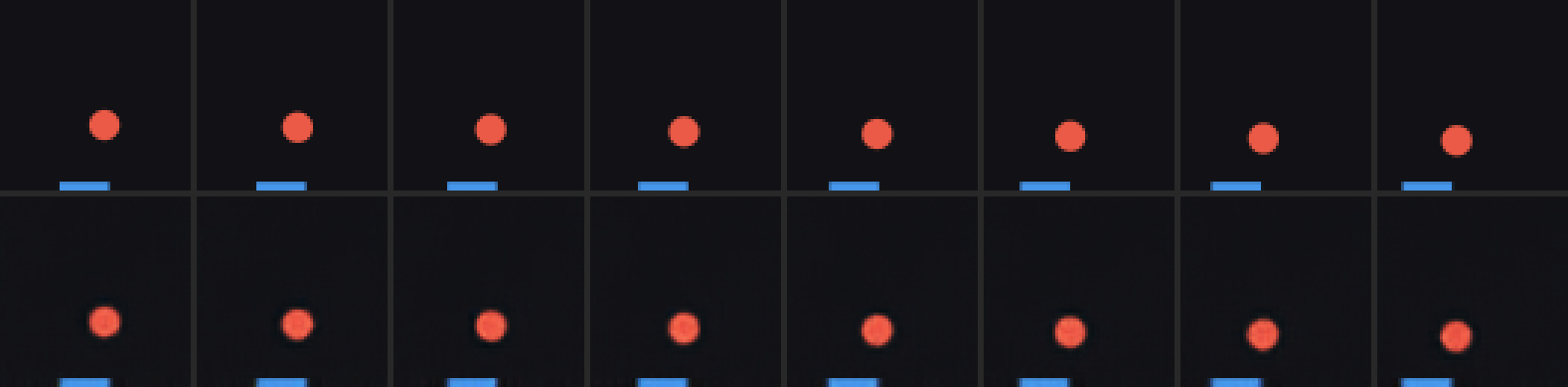
Top row: real frames. Bottom: decode(μ). The ball is present, correctly placed, slightly softer-edged. The paddle is essentially perfect. This is the prerequisite for everything: if this row were mush, no downstream result would be interpretable.
6.2 Probes — is the true state recoverable from z?
We fit regressors from μ to each true state variable, on a held-out
episode-level split (so no test frame has a near-twin in the train set).
R² = 1 means perfectly recoverable, 0 means no better than predicting the mean.
| variable | linear | poly-2 | poly-3 | kNN | MLP |
|---|---|---|---|---|---|
| ball_x | 0.04 | 0.98 | 0.99 | 0.99 | 0.98 |
| ball_y | 0.22 | 0.97 | 0.99 | 0.98 | 0.98 |
| paddle_x | 0.70 | 0.98 | 0.99 | 0.59 | 0.98 |
| ball_vx | < 0 | < 0 | < 0 | < 0 | < 0 |
| ball_vy | < 0 | < 0 | < 0 | < 0 | < 0 |
| paddle_vx | < 0 | < 0 | < 0 | < 0 | < 0 |
Three conclusions, in decreasing order of obviousness:
- Positions are in
z, almost perfectly (R² ≈ 0.99). The information survived the bottleneck. - Velocities are not in
zat all, and this is correct. A single frame is pixel-identical whether the ball is moving up or down. Velocity is not a property of a frame; it is a property of a pair of frames. If we had seen a high velocity R² here it would have meant a leak, not a success. This is the cleanest possible demonstration of why the world-model recipe has an M stage: something has to integrate over time, and V by construction cannot. - The code is nonlinear. Linear R² for ball position is ~0.04–0.2 while kNN and polynomial probes hit 0.99. The information is there, but not as “dimension 3 = x-coordinate”. The next two pictures show what it is instead.
6.3 Latent traversals — what does each dimension do?
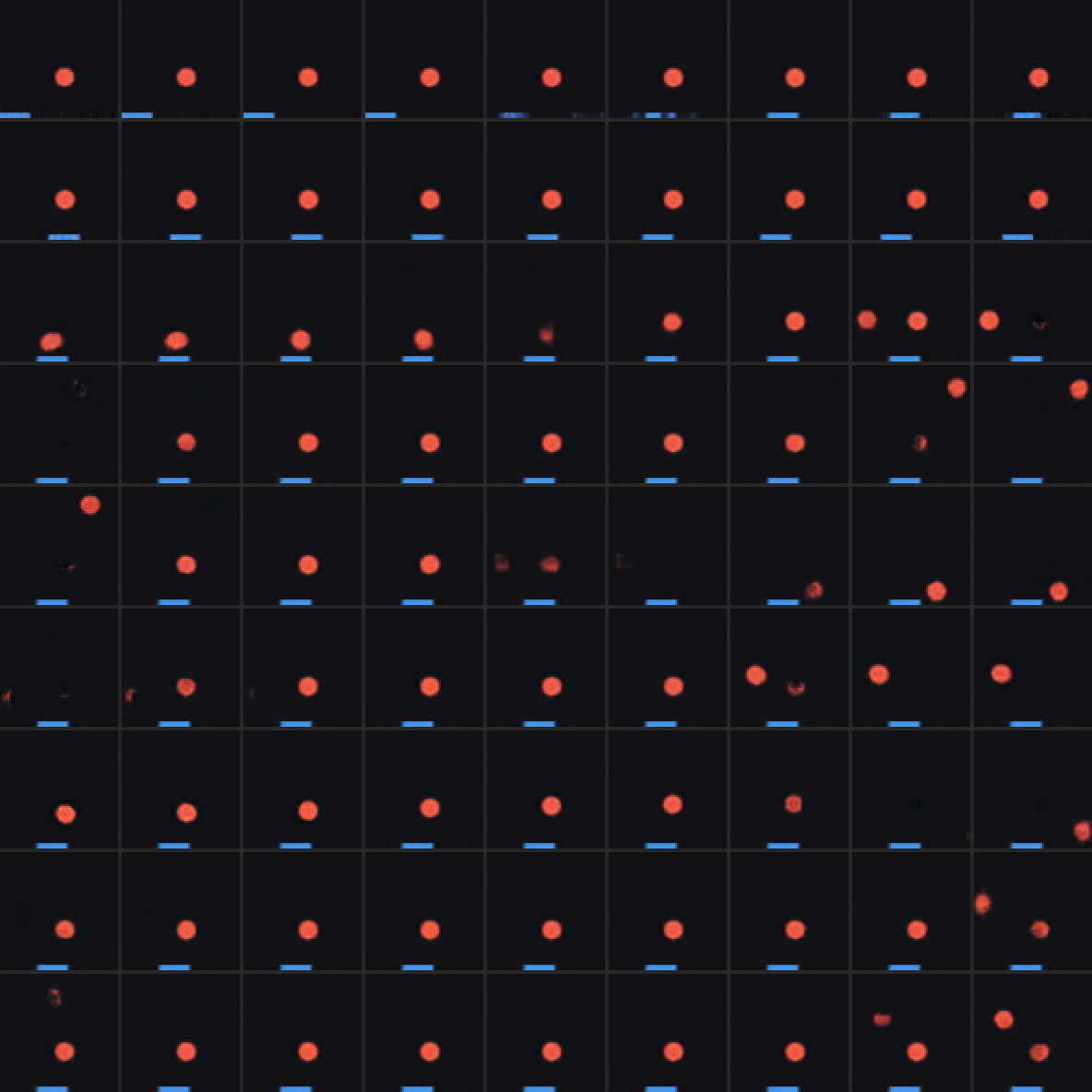
Each row sweeps one active dimension from −3σ to +3σ with the others held fixed. In a textbook “disentangled” VAE one row would slide the ball horizontally and another vertically. Here, instead, sweeping a dimension makes the ball fade out at one location and fade in at another, sometimes briefly showing two balls. Some rows barely change the image within the central range and only act at the extremes.
That is the signature of a localised, place-cell-like code: individual dimensions behave like “is the ball near region R?” detectors rather than coordinates.
6.4 Tuning maps — the decisive plot
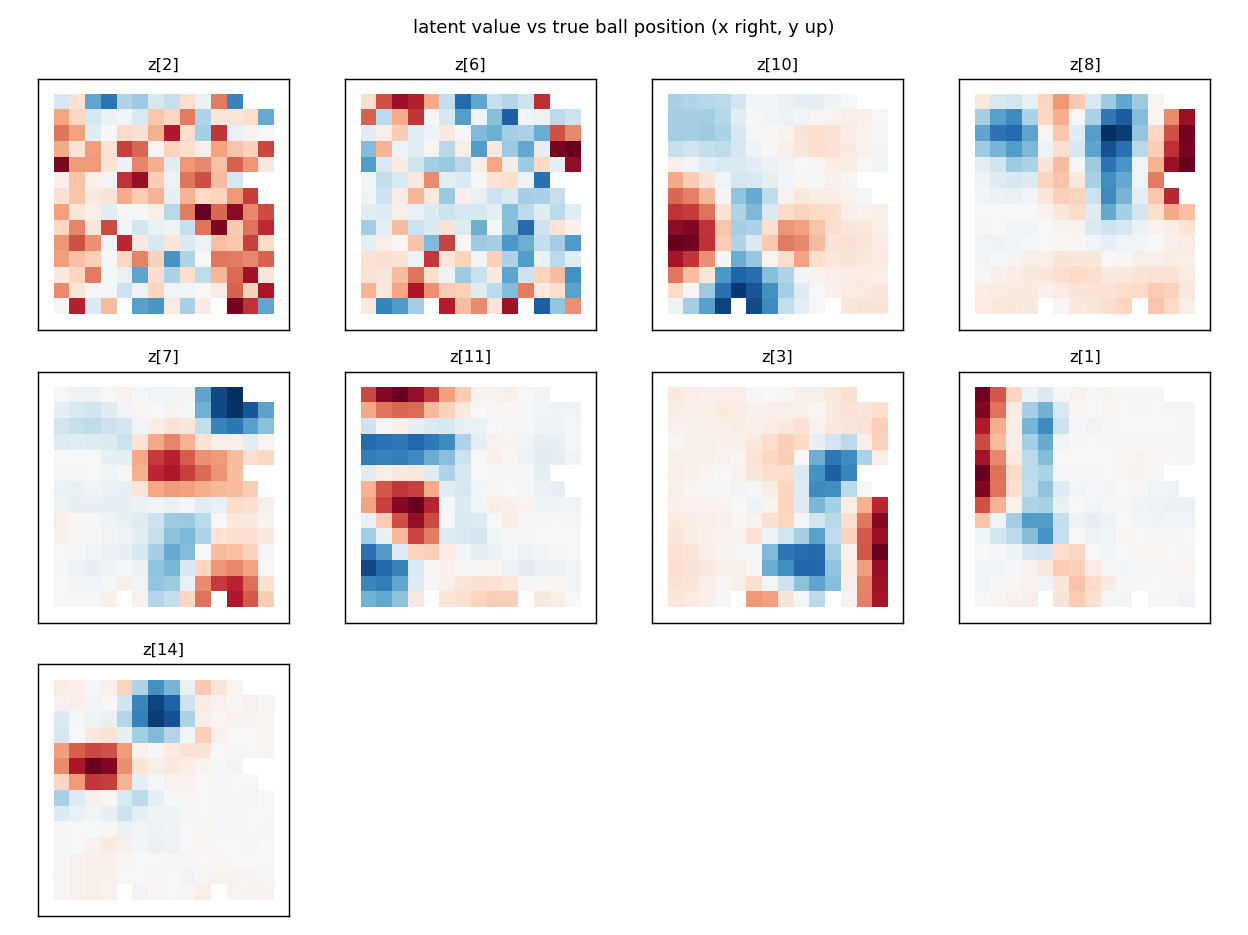
Each panel is one latent dimension; the colour at (x, y) is the average value of that dimension when the true ball is at (x, y). A coordinate-like code would be a smooth left-to-right (or bottom-to-top) ramp. What we see:
z[10],z[7],z[14],z[3]: blobs — the dimension fires when the ball is in one or two specific regions. Place fields.z[11],z[1],z[8]: stripes — periodic in y or x, i.e. the dimension encodes something likecos(k·π·y).z[2],z[6]: speckle, no ball-position structure. These dimensions are about the paddle (linear paddle_x R² = 0.70 confirms at least one is).
Position is therefore encoded jointly across ~7 dimensions as a set of
overlapping bumps and stripes — which is why any single-dimension or linear
readout fails and any smooth nonlinear one succeeds. wm/calibrate_probes.py
confirms this reading by running the same probes on synthetic codes of known
form: narrow place fields and k ≥ 2 Fourier codes produce exactly this
“linear low / kNN high” pattern.
Is this bad? Not for reconstruction, and not for a kNN reader. It is less
convenient for the dynamics model: physics is linear-ish in (x, y) — x_{t+1}
= x_t + v_x — but in a place-field code the same motion is a complicated
rotation among many dimensions. M will have to learn that. We keep this
checkpoint on purpose: seeing how well M copes with a realistic, non-ideal
latent space is more instructive than engineering an ideal one first.
Why did it happen? Convolutional features are inherently local detectors (“something red here”), and the flatten→Linear layer has no incentive to convert them into coordinates when a mixture of local detectors reconstructs just as well. Getting axis-aligned coordinates out of a VAE generally needs extra pressure (β-VAE / higher β, TC penalties, or supervision), each of which trades off reconstruction sharpness. That is the disentanglement literature in one sentence, and a clear candidate for a v1.1 experiment.
6.5 Prior samples — will the decoder tolerate imperfect z?
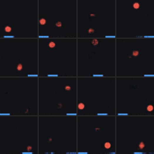
Decode 16 draws of z ~ N(0, I). Most produce a plausible frame: one ball,
one paddle, dark background. A few produce a faint or doubled ball, or a paddle
fragment. This matters for M: dreamed latents will wander off the data manifold
a little, and this picture says the decoder degrades gracefully rather than
catastrophically. If these were noise, no dream rollout could survive more than
a few steps regardless of how good M was.
6.6 MCC — recovery up to permutation?
Mean Correlation Coefficient (the identifiability-literature metric) is 0.33 Pearson, 0.31 Spearman. Low, and expected given the above: MCC asks whether each true factor maps to one latent dimension by a monotone function. A place-field code fails that test by construction even though the information is fully present. Read MCC alongside the probes, never alone.
7. What was achieved, and what to remember
Achieved. A frozen encoder that maps frames to a 16-d code from which ball and paddle positions are recoverable to ~1% of the box width, whose decoder draws sharp, correctly placed objects, and whose latent space is smooth enough that random prior samples look like game frames. That is a sufficient V for the Ha & Schmidhuber recipe.
Remember.
- Velocity R² ≈ 0 from a single frame is the correct answer and is the motivation for M.
- Global pixel loss lies on small-object worlds. Track masked error and probes.
- Posterior collapse is the default outcome here; free bits + warm-up is the fix.
- The VAE learned a distributed place-field code, not coordinates. Nonlinear probes recover the state; linear ones do not. This is the latent space M has to do physics in.
- Latents are cached once (
wm/cache_latents.py) — 425 MB of frames become ~4 MB of(μ, log σ²)— and V is never fine-tuned jointly with M, so every later result is attributable to M alone.
Next: 03 — M: the dynamics model.