03 — M: the dynamics model (an MDN-RNN that dreams)
How the world model learns physics from a stream of latent codes, how we check that it did, and what it got right and wrong.
1. The job of M in one sentence
Given what the frame looks like now (z_t), what the agent does now (a_t),
and what M remembers about the recent past (h_t), predict what the next
frame will look like (z_{t+1}).
That is the whole of “learning physics” in this recipe. Nothing is told to the model about balls, walls, velocity or collisions. It sees 16-number codes arriving one per frame and has to find the rule that generates the next one.
Once it can do that for one step, it can do it for many: feed its own prediction back in as the next input, and it produces a whole imagined future — a dream. Decoding each dreamed code with V’s decoder turns that into a video we can watch and grade.
2. Three design decisions, and the reason for each
The model is in wm/rnn.py (about 330k parameters). Every
non-obvious choice is also annotated inline in the source.
2.1 Why recurrent — where velocity has to live
Doc 02 established that a single code z_t contains position but no
velocity (probe R² ≈ 0). So z_{t+1} is not a function of (z_t, a_t)
alone: the same frame can be followed by the ball going up or down. The
transition is not Markov in z.
A recurrent network fixes that by carrying a hidden state h_t from step to
step. If it wants to predict well, it must learn to store in h_t whatever
the current frame lacks — above all, which way the ball is moving. Section 5.3
tests that claim directly.
We use a single-layer LSTM with 256 units, as in the paper. Depth is not the hard part here; carrying information through time is.
2.2 Why a mixture density output — the averaging failure
The obvious output layer predicts one z_{t+1} and is trained with squared
error. That is a single Gaussian with fixed variance, and it has a specific,
fatal weakness: when the future is genuinely uncertain — two frames before the
ball reaches the floor, will it hit the paddle or miss? — the squared-error
optimum is the average of the possible futures. A ball “in between” the
bounce and the miss, a place the ball can never be. In a one-step metric this
looks fine. In a rollout it is fatal, because the averaged state is off the
data manifold and the next prediction is garbage.
A Mixture Density Network (MDN) head instead outputs K = 5 Gaussians —
weights, means, standard deviations — so the model can put mass on “bounces”
and on “misses” and, when sampled, commit to one. The loss is the negative
log-likelihood of the true z_{t+1} under the mixture, computed entirely in the
log domain with logsumexp (the naive product of densities underflows to zero
in 16 dimensions and the run dies).
Setting K = 1 recovers a plain Gaussian regression, so the comparison is a
one-flag change. We ran it (§5.1).
2.3 Why predict the change — residual dynamics
Consecutive codes are very similar: the ball moves 0.022 of the box per frame.
Predicting z_{t+1} directly means the network must first learn to copy its
input to high precision before any capacity goes to physics. So the MDN models
the residual z_{t+1} − z_t, and the input is added back. The network
starts life as the identity map (a decent predictor already) and only has to
learn the change.
2.4 Two extra heads
Off the same hidden state we attach two tiny linear heads:
- hit: the probability that this transition is a paddle contact (trained with a class-weighted cross-entropy, because contacts are <1% of transitions and an unweighted loss is minimised by “never”).
- reward: a dense shaping reward
1 − |ball_x − paddle_x|of the next state.
These cost nothing and are what turn M into a usable environment for the controller in doc 04: a policy can dream forward and be told how well it is doing, without touching the real simulator. The reward target is computed from the simulator’s true state — exactly as a real environment computes reward — and is never an input to the model.
3. Training
Code: wm/seq_data.py, wm/train_rnn.py.
python -m wm.train_rnn --data data/v1/train data/v1/train_mix \
    --val data/v1/val data/v1/val_mix --out runs/rnn_v1 --epochs 35 --eval-every 2
- Data: the cached VAE posteriors for
train(150 episodes, random policy) plustrain_mix(300 episodes, half tracking / half random — see doc 01 §5), cut into windows of 32 transitions that never cross an episode boundary. About 90k transitions per epoch. - Inputs are sampled, not means. Every time a window is fetched we draw
z = μ + σ·εfresh from the cached posterior. Two reasons: it is free data augmentation, and — more importantly — at dream time the model is fed its own samples, which are noisy. Training on clean means would give a model that has never seen the input distribution it faces in a rollout. - Teacher forcing: during training the model always receives the true
z_tand predicts one step ahead. This is fast and stable, but note what it hides: errors never compound, because every step is corrected by the truth. Open-loop rollout error — the thing we actually care about — has to be measured separately, so the trainer runs a 32-step open-loop rollout on validation data every two epochs and logs it alongside the loss. - Adam, learning rate 1e-3, gradient clipping at 1.0, 35 epochs, ~20 s per epoch on the M1’s CPU (the GPU was 4× slower: a 256-unit LSTM stepped 32 times is a chain of tiny matrix multiplies, bound by dispatch latency rather than arithmetic).
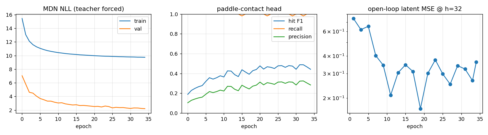
Two things in that figure are worth internalising.
Train and validation NLL are not comparable (9.7 vs 2.2). Training targets are posterior samples, validation targets are posterior means. The sampled target carries the VAE’s own posterior noise and is genuinely harder to predict. This looked alarming until it was traced.
Teacher-forced loss kept improving after dream quality stopped. The validation NLL falls steadily from epoch 12 to 35 (2.9 → 2.2). The open-loop rollout error (right panel) bottoms out around epoch 12 and then just fluctuates. The last twenty epochs bought better one-step predictions and essentially no better dreams. This is the classic gap in dynamics-model training, and it is why the rollout metric lives inside the training loop rather than only in a post-hoc evaluation.
3.1 Controls
Two additional models were trained with identical data and budget:
| run | change | best val NLL | open-loop latent MSE @ 32 steps |
|---|---|---|---|
runs/rnn_v1 |
main: K=5 mixture, residual | 2.21 | 0.36 |
runs/rnn_g1 |
K=1 (plain Gaussian) | 2.25 | 0.19 |
runs/rnn_noact |
action input zeroed | 3.23 | 0.64 |
- Zeroing the action costs a full nat of NLL. The model demonstrably uses the action. (§5.4 shows what it uses it for.)
- The mixture barely beats the Gaussian on likelihood, and the Gaussian rolls out more accurately in latent space. This was not expected and is reported as-is. Two plausible, undisentangled reasons: validation targets are posterior means, which strips out much of the multimodality the mixture exists to model; and at temperature 0 the mixture rollout commits to its highest-weight component each step, and component-switching between steps makes the trajectory less smooth than a unimodal model’s. This is a good first follow-up experiment. It also illustrates a general lesson: the textbook argument for a design choice (§2.2) can be correct and not matter on a given problem.
4. How a dream is made and graded
Code: wm/eval_rnn.py. Everything below is written to
runs/rnn_v1/eval/.
python -m wm.eval_rnn --ckpt runs/rnn_v1/rnn.pt --vae runs/vae_b1/vae.pt \
    --val data/v1/val data/v1/val_mix --out runs/rnn_v1/eval
Procedure. Take a real validation episode. Feed the model the first 8 true
codes with the true actions — a warm-up so h acquires velocity. Then cut
the model off from the truth: for the next 64 steps it receives the true
action (so we grade physics, not the agent) but its own predicted code,
sampled from the mixture at a chosen temperature τ. Decode every dreamed
code with V’s decoder.
Temperature. τ multiplies the predicted standard deviations and sharpens the mixture weights. τ = 0 means “always take the mean of the most likely component” — a deterministic, reproducible dream. τ = 1 samples from the model’s honest predictive distribution. Both are reported below; they answer different questions.
Grading in world coordinates. Pixel error is a poor yardstick (doc 02 §4), so we also read the dreamed code back into world coordinates: a k-nearest- neighbour regressor from VAE codes to true state, fit on separate data and frozen, is applied to the dreamed codes. That gives “where the model thinks the ball is” as an (x, y) pair, to be compared against where the ball really was. The probe’s own error on true codes (about 0.004 of the box for the ball) is the floor.
An honest footnote. The first version of this evaluation compared dream step
k with the true state at step k+1 — an off-by-one that charged the model one
frame of ball motion at every horizon. It was caught in review because the
one-step pixel error was implausibly 12× the VAE floor. Corrected, it is 1.8×.
Alignment bugs in sequence evaluation are common and quiet; the fix and the
original numbers are recorded in wm/README_M.md.
5. Results — what M learned
5.1 Dreams vs reality

Top row: the real episode. Middle: V’s reconstruction of the true codes (the
best the decoder could possibly show). Bottom: the τ = 0 dream. The dreamed
ball descends, reaches the floor, and comes back up in step with the real one;
the paddle follows the real actions. Animated versions:
dream_vs_true_tau0.0.gif, …tau0.5.gif, …tau1.0.gif.
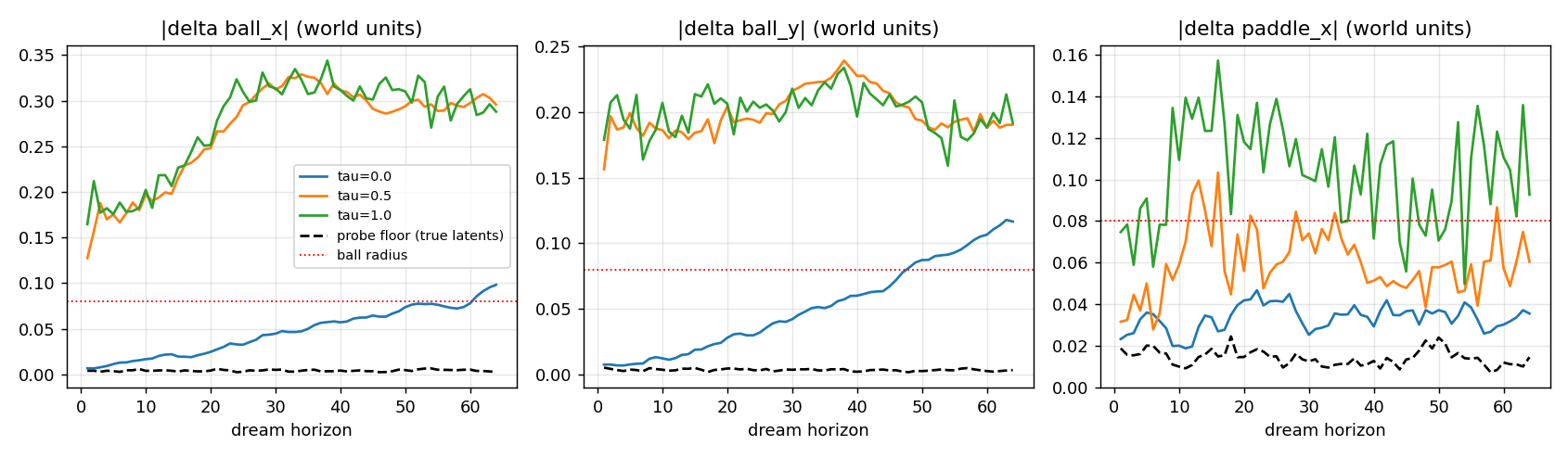
| horizon (steps after warm-up) | 1 | 16 | 35 | 64 |
|---|---|---|---|---|
| dreamed ball position error, τ = 0 (box widths) | 0.012 | 0.019 | 0.08 | 0.16 |
| probe floor on true codes | 0.004 | 0.004 | 0.004 | 0.004 |
We call the horizon at which the dreamed ball has drifted more than one ball radius (0.08) from the real one the useful dream horizon: 35 steps, or about one and a half seconds of game time at 20 fps, or roughly one full wall- to-wall traverse of the box. Error grows roughly linearly, which is what a small velocity error integrated over time looks like — not the exponential blow-up of a model that has lost the plot.
The τ > 0 curves score zero on this metric, and that is mostly the metric’s fault. A sampled dream is a different plausible future, not a failed copy of this one. Look at the τ = 1 contact sheet: the ball is still round, moves smoothly and bounces — it is just not doing what this particular real ball did. The large one-step error at τ = 1 (0.17) has a specific cause: the model was trained on posterior samples, so its predictive spread correctly includes the VAE’s own posterior noise, which in 16 dimensions is large. For grading physics, use τ = 0. For training a controller, the paper’s argument is the opposite — a wider dream is harder to exploit — and doc 04 takes that up.
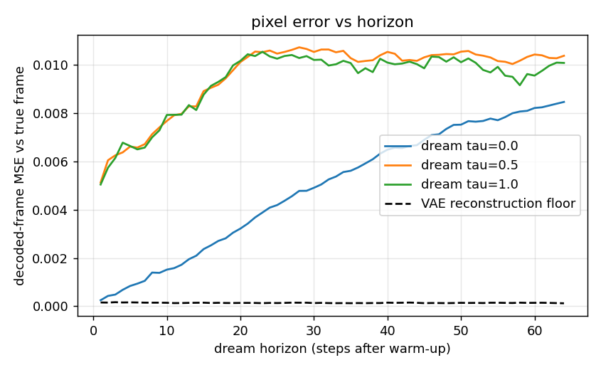
The pixel view tells the same story: the τ = 0 dream starts within 2× of the VAE’s own reconstruction floor and drifts away roughly linearly.
5.2 Does it know about walls?
The weakest of our tests. We find validation moments just before a wall bounce, dream through them, and ask whether the dreamed ball sustainedly reverses within ±2 steps of the real bounce. It does in 36.5% of 200 cases; applying the same detector at a random time in the same dream scores 15.5%. Better than chance, clearly not mastery. Two caveats: the detector is crude (any reversal on either axis), and the τ = 0 dream in the contact sheet visibly does bounce off the floor. A per-wall, per-axis version of this test is an obvious improvement.
5.3 Where does velocity live? — the central result
We run the model teacher-forced over validation episodes, collect the hidden
state h_t at every step, and ask the same probe question as in doc 02, three
times: from z_t alone, from h_t alone, and from both.
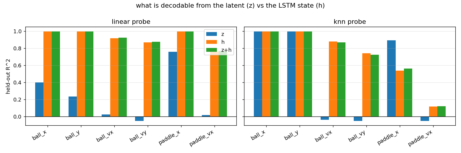
Held-out R², linear probe:
| from | ball_x | ball_y | ball_vx | ball_vy | paddle_x | paddle_vx |
|---|---|---|---|---|---|---|
z (the frame code) |
0.40 | 0.23 | 0.02 | −0.11 | 0.76 | 0.02 |
h (the LSTM state) |
0.995 | 0.994 | 0.92 | 0.87 | 0.994 | 0.76 |
This is the cleanest single picture of what the world model has done:
- Velocity is absent from the frame code and present in the memory. Nobody told the LSTM about velocity. It discovered that storing the ball’s direction of travel is what it takes to predict the next frame, and it stores it in a form a linear readout can recover.
- The LSTM also re-coded position linearly. From
z, ball position was recoverable only by a nonlinear probe (the place-field code of doc 02, kNN R² 0.99 but linear 0.04). Fromh, a linear probe gets 0.995. The recurrent network has effectively unfolded V’s curved code into something coordinate-like — presumably because linear dynamics are easiest to implement on a linear representation. That is a small, unplanned demonstration of a big idea: representations get shaped by what they are used for. paddle_vx(0.76) is lower than ball velocity because the paddle is stationary in a large fraction of frames and clamps at the walls; it is a noisier target.
5.4 Does it know actions matter? — counterfactual dreams
From the same warm-up, dream three futures: always-left, always-stay, always-right. Nothing else differs.
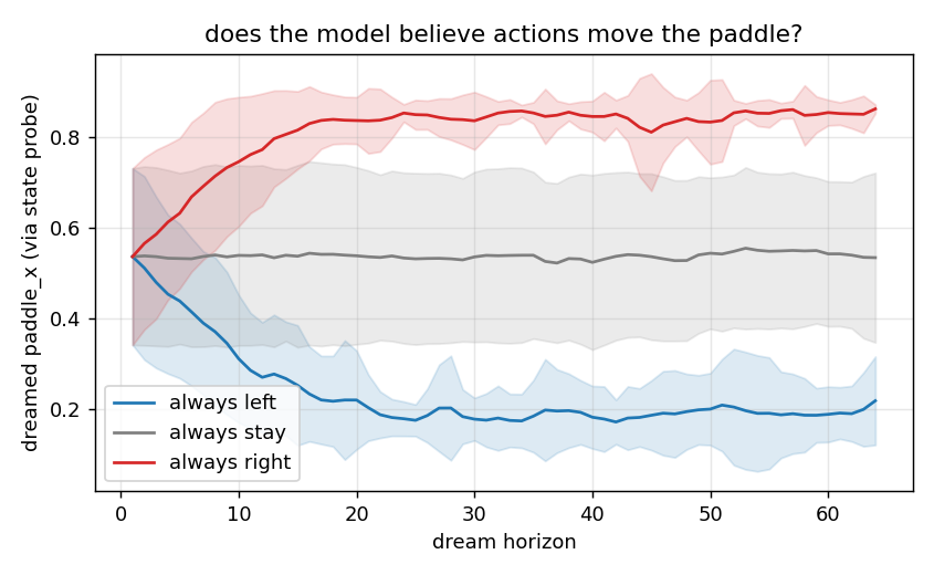
The dreamed paddle slides left or right and saturates at 0.13 and 0.87 —
which are exactly the simulator’s clamp limits (half a paddle width from each
wall). The model learned not just that actions move the paddle but where the
paddle stops. Mean separation between the left and right dreams after 30
steps: 0.66 of the box. The action-ablated control model: 0.00, by
construction. The animated version, action_counterfactual.gif, shows three
side-by-side dreams diverging from an identical start — the closest thing in
this project to watching a model reason about “what if”.
Note what this test does not show: whether the model knows the paddle deflects the ball. That effect is contact-mediated and rare (doc 01 §3), and the next diagnostic is the closest we get to it.
5.5 Anticipating contact
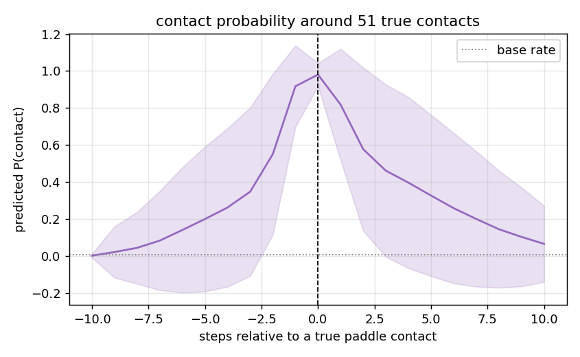
Average predicted contact probability, aligned on the 51 real paddle contacts in
the validation set. The base rate is 0.7%. Three steps before a contact the
model already says 35%; one step before, 92%. It is not merely recognising a
collision after the fact (that would be a spike at lag 0 and nothing before):
it is extrapolating the ball’s trajectory to the paddle’s position, which
requires exactly the velocity information in h. Threshold-free quality:
PR-AUC 0.73 against a chance level of 0.007. (The wide band is 51 events; more
validation episodes would tighten it.)
6. What was achieved, and what to remember
Achieved. A dynamics model that, from 16-number frame codes alone, learned to carry velocity in its memory, predicts the paddle’s response to actions including its limits, anticipates paddle contacts several frames early, and produces deterministic dreams that track reality for ~35 frames. Together with V, it is a complete, inspectable simulator of the game learned from pixels — the thing doc 04 trains an agent inside.
Remember.
- Velocity is not in a frame. A recurrent state is where it must go, and
probing
his how you check it went there. - Teacher-forced loss can keep falling while dream quality does not. Always measure open-loop rollouts, preferably in world coordinates, not pixels.
- Deterministic (τ = 0) dreams are for grading physics. Sampled dreams are different futures and should not be graded by agreement with one real one.
- Counterfactual dreams are the most direct test of a learned causal channel: same start, different action, compare outcomes.
- A textbook-justified choice (the mixture head) did not measurably help here. Run the ablation; do not assume.
- Alignment bugs in sequence evaluation are silent. Sanity-check the one-step error against a floor you trust.
Open threads. Why the Gaussian rolls out better than the mixture; a proper
per-wall bounce test; whether training on posterior means (--use-mean)
narrows the τ = 1 dream without hurting robustness; and a transformer in place
of the LSTM for the long-range dependencies planned in v4.