V2 stage one — the vision model on mass-from-colour
Technical log for the v2 VAE. Environment side is documented in
worldsim/worldsim.md; read
that first, then this. For the v1 VAE and the conceptual background see
docs/02_vae_the_vision_model.md — the
architecture, the free-bits story and the posterior-collapse failure mode are
all unchanged here.
The one-sentence question for stage one of v2: in v1, z carried positions
and nothing else; now that the ball’s colour determines its mass, does z carry
the colour, and in what form?
The answer, up front. Yes, and it is worth more than it looks. The decoder
reproduces the colour faithfully (median 6.3% error in the mass you can read
back out of a reconstruction, rank correlation 0.98). mass, log_mass and
|v| are all recoverable from a single frame’s mu at R² ≈ 0.91 / 0.97 / 0.98
with a degree-2 probe, while ball_vx and ball_vy stay firmly undecodable, as
in v1. And the whole thing cost about 1 extra nat of KL, spent on a code
that is distributed — no single latent dimension carries colour.
Scoring the V-stage predictions from docs/v2/00_v2_design.md
| prediction | outcome |
|---|---|
mass R² > 0.9 from z |
yes — 0.910 (poly-2), log_mass 0.972 |
speed decodable from a single frame while vx,vy are not |
yes — 0.975 vs < 0 |
| one more active latent dimension than v1 (~10) | no — 8 by the same threshold, 6 clearly active. Colour went inside existing dimensions, not beside them (§5.5) |
| mass decoding interpolates into the held-out band | partly — correct to ±0.11 in mass on a 0.5–2.0 scale, but no resolution within the band (§6) |
1. Commands, in order, with wall clock
Everything ran on the M1 (8 GB) with python.
# data -- 40 s total, 1.3 GB
COMMON="--ball-radius 0.08 --steps 200 --res 64 --mass-from-color"; HO="--mass-holdout 0.85 1.2"
python -m worldsim.collect --out data/v2/train     --episodes 150 --seed 0   --policy sticky $COMMON $HO
python -m worldsim.collect --out data/v2/train_mix --episodes 300 --seed 10  --policy mix --p-track 0.5 $COMMON $HO
python -m worldsim.collect --out data/v2/val       --episodes 15  --seed 1   --policy sticky $COMMON $HO
python -m worldsim.collect --out data/v2/val_mix   --episodes 20  --seed 11  --policy mix $COMMON $HO
python -m worldsim.collect --out data/v2/probe     --episodes 120 --seed 777 --policy sticky \
    --steps 24 --ball-radius 0.08 --res 64 --mass-from-color $HO
python -m worldsim.collect --out data/v2/holdout   --episodes 30  --seed 21  --policy mix $COMMON --mass-only 0.85 1.2
python -m worldsim.v2_figures --data data/v2/train --gif-data data/v2/val_mix --out runs/v2_env   #  6 s

# the VAE -- 17 min for 60 epochs on mps
python -m wm.train_vae --data data/v2/train --val data/v2/val --out runs/vae_v2 \
    --epochs 60 --z-dim 16 --free-bits 0.5 --warmup-epochs 5 --device mps --eval-every 10

# analysis -- 68 s
python -m wm.analyze --ckpt runs/vae_v2/vae.pt --data data/v2/probe \
    --eval-data data/v2/holdout --tuning-data data/v2/train_mix \
    --device mps --out runs/vae_v2/analysis

# latents for stage two -- ~20 s per split
for d in train train_mix val val_mix probe holdout; do
  python -m wm.cache_latents --ckpt runs/vae_v2/vae.pt --data data/v2/$d --device mps
done

# tests -- 9 s
python -m pytest tests/ -q         # 34 passed (11 of them the new test_env_v2)
Training was budgeted at up to 45 minutes; 60 epochs came in at 17 min
(17 s/epoch), i.e. considerably faster than the v1 run quoted in docs/02
(54 min for 80 epochs). Same model, same data size — the difference is machine
load, not anything about v2. No need to cut to 50 epochs.
2. Data
| split | eps × steps | policy | contact rate | mean effective speed | mass range |
|---|---|---|---|---|---|
train |
150 × 200 | sticky | 0.553% | 0.0230 | 0.50–1.99, gap 0.85–1.2 |
train_mix |
300 × 200 | mix p=0.5 | 0.843% | 0.0253 | 0.50–1.99, gap |
val |
15 × 200 | sticky | 1.067% | 0.0252 | 0.57–1.93, gap |
val_mix |
20 × 200 | mix | 0.675% | 0.0242 | 0.51–1.94, gap |
probe |
120 × 24 | sticky | 0.521% | 0.0258 | 0.50–2.00, gap |
holdout |
30 × 200 | mix | 1.133% | 0.0219 | 0.89–1.19 only |
Full log-binned mass histograms per split are in runs/v2_env/collect.log.
They are flat on a log axis with an empty [0.891, 1.122) bin, which is the
hold-out band showing up exactly where it should. Paddle-contact rates are 2–5×
the v1 figure (~0.2%) — partly the larger ball (--ball-radius 0.08) and partly
that light balls reach the floor far more often per episode.
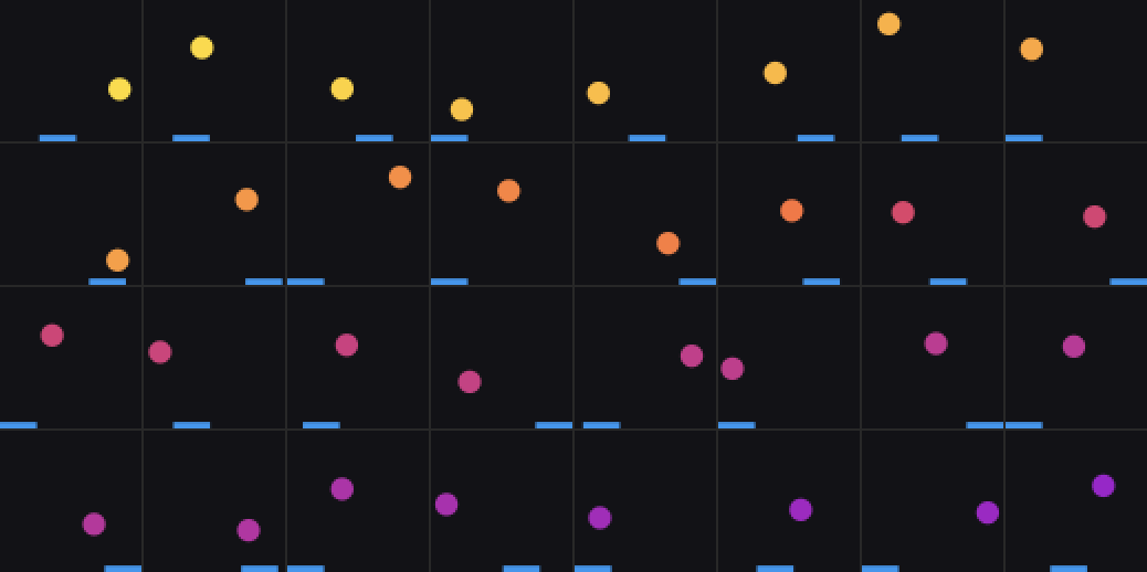
The missing red band in the middle of that ramp is the generalisation test.
3. Training curve
runs/vae_v2/history.json, runs/vae_v2_train.log.
| epoch | loss | KL (nats) | global MSE | ball MSE | active units |
|---|---|---|---|---|---|
| 0 | 201.4 | 245.4 | 0.0158 | 0.0936 | — |
| 4 | 32.5 | 18.3 | 0.00131 | 0.0161 | — |
| 9 | 27.3 | 16.7 | 0.00086 | 0.0103 | 12 |
| 19 | 23.8 | 16.0 | 0.00063 | 0.0077 | 11 |
| 29 | 22.5 | 15.7 | 0.00054 | 0.0066 | 10 |
| 39 | 21.7 | 15.6 | 0.00049 | 0.0061 | 10 |
| 49 | 21.2 | 15.5 | 0.00046 | 0.0057 | 9 |
| 59 | 20.8 | 15.5 | 0.00043 | 0.0053 | 9 |
Read against v1 (KL 14.4, global MSE 0.00036, ball MSE 0.0042 at epoch 79):
- KL settles at 15.45 vs v1’s 14.4 — about one extra nat for colour. One nat is ~2.7 distinguishable levels if you spend it naively, but the encoder is not transmitting colour independently of everything else, and the probes below say the effective resolution is far finer than that. Still, it is a useful reminder of how cheap this variable is compared to position (~8 nats).
- Ball-region MSE is ~12× the global MSE, same ratio as v1. The extra colour variance did not make the ball harder to draw.
- The run had not fully plateaued at 60 epochs (loss still dropping in the third decimal), but the probe numbers were stable from epoch 30 on.
4. Reconstructions: is the colour preserved?
This was the designated v2 failure mode — a model that renders every ball the same average orange would be a total failure of the point of v2 while barely moving the loss, exactly as v1’s “ball missing entirely” failure barely moved the loss.

Top row: real frames from 16 episodes spanning the mass range, sorted light to
heavy. Bottom row: decode(mu). The ramp survives.
Quantitatively (color_fidelity in wm/analyze.py — decode, find the most
ball-like pixel, run it back through worldsim.color_to_mass):
median |Δm|/m = 0.063 max 0.199 spearman(true, decoded) = 0.982
analysis/prior_samples.png (decode z ~ N(0, I)) is also healthy: plausible
frames, a ball and a paddle, and colours spread across the ramp rather than all
one hue — so the aggregate posterior has spread the colour axis over the prior
too, which is what dream rollouts in stage two will need.
Note that the routine recon.png grid cannot answer this question: its
eight frames come from one episode and therefore share one mass. Checking colour
fidelity needed a grid that varies the right variable, which is a small lesson
in its own right — a diagnostic inherited from the previous stage can be
silently blind to the new stage’s whole point.
5. Probes: what is in mu?
runs/vae_v2/analysis/report.json. Probe set = 120 episodes × 25 frames,
held-out episode-level split.
| variable | linear | poly-2 | poly-3 | kNN | MLP |
|---|---|---|---|---|---|
| ball_x | 0.491 | 0.876 | 0.952 | 0.916 | 0.956 |
| ball_y | 0.342 | 0.796 | 0.951 | 0.950 | 0.951 |
| paddle_x | 0.662 | 0.962 | 0.989 | 0.773 | 0.990 |
| ball_vx | −0.12 | −0.42 | −2.27 | −0.35 | −0.60 |
| ball_vy | −0.15 | −0.32 | −1.84 | −0.48 | −0.62 |
| paddle_vx | −0.01 | −0.25 | −1.20 | −0.29 | −0.43 |
| mass | −0.385 | 0.910 | 0.861 | 0.088 | 0.888 |
| log_mass | −0.430 | 0.972 | 0.962 | 0.083 | 0.950 |
| speed | −0.451 | 0.975 | 0.988 | 0.065 | 0.934 |
Positions behave exactly as in v1: present, but in a nonlinear code. Velocities are absent, also exactly as in v1, and that remains the correct answer — a single frame is pixel-identical whether the ball moves up or down.
5.1 The v2 headline: speed is decodable but ball_vx/ball_vy are not
speed = |v| = ball_speed / m, so it is a pure function of colour. The frame
shows no motion whatsoever, yet R²(speed) = 0.975 while both of its own
components sit below zero. That is not a contradiction, it is the appearance →
dynamics causal edge appearing at stage V:
V cannot see motion. V can see colour. In v2, colour determines the magnitude of motion. So the vision model, trained on shuffled single frames with no notion of time, has nonetheless acquired information about the dynamics.
This is worth sitting with before stage two, because it changes what M has to
do. In v1, M had to integrate observations over time to recover velocity from
nothing. In v2, M gets a strong prior on |v| for free from z alone and has to
learn only the direction, plus the fact that this latent multiplies the
per-step displacement. That multiplication is a genuinely new demand: it is an
interaction between two latents, which no linear dynamics model can express.
log_mass scores slightly higher than mass (0.972 vs 0.910 at poly-2), which
is the expected sign: the pixels vary linearly in u ∝ log m, so the latent
code is closer to log-mass than to mass, and the extra 1/m warp costs a little.
5.2 The pattern that surprised me: poly-2 ≈ 0.97 but kNN ≈ 0.08
For every position variable in v1 and v2, kNN was at least as good as the polynomial probes — the usual “the information is there, under some smooth map” upper bound. For mass it collapses to nothing while poly-2 is nearly perfect.
The explanation is about geometry, not about missing information. kNN measures
Euclidean distance in standardised mu, and mu’s variance is overwhelmingly
positional. So the ten nearest neighbours of a frame are ten frames with a
similar ball position, drawn from ten episodes with ten different masses, and
their average mass is just the dataset mean. A polynomial probe, by contrast,
can find the specific low-variance direction (or curved surface) along which
colour varies and ignore everything else.
Practical lesson: kNN is an upper bound on decodability only for factors that are prominent in the latent metric. For a low-variance factor entangled with a high-variance one it is a lower bound and a misleading one. Read it as “is this factor a dominant axis of the latent geometry”, not “is this information present”.
5.3 MCC and where colour lives
MCC pearson 0.276   spearman 0.282
  ball_x   -> z[ 8]  |r|=0.420      paddle_x  -> z[ 7]  |r|=0.774
  ball_y   -> z[ 9]  |r|=0.353      mass      -> z[13]  |r|=0.150
  ball_vx/ball_vy/paddle_vx -> |r| < 0.09  (nothing to match)
Low, for the same reason as v1: MCC is a linear statistic and this code is nonlinear, so MCC cannot distinguish “did not recover” from “recovered under a nonlinear map”. The mass row (|r| = 0.15 Pearson, 0.34 Spearman) is the interesting one — rank correlation more than doubles the Pearson value, so whatever single-dimension colour signal exists is monotone but strongly curved.
5.4 Is there a “colour dimension”? No.
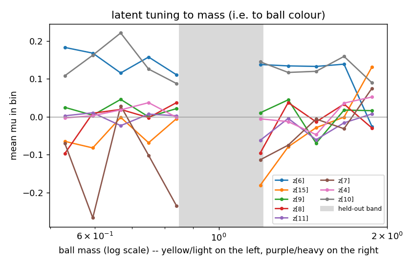
Mean mu per log-mass bin, for the eight most-informative dimensions, computed
on 40k frames of train_mix (the probe set’s 120 × 24 frames is not enough for
the positional variance to average out — the first version of this plot was
mostly noise, which is why --tuning-data exists). Grey band = the masses the
VAE never saw.
Two dimensions (z[7], z[15]) look like they slope. But the decisive test is a
probe restricted to one dimension at a time — held-out R² for log_mass from
z[d] alone:
z[9] -0.108 z[11] -0.117 z[8] -0.193 z[15] -0.201 z[4] -0.204 z[6] -0.254 z[7] -0.285
Every single dimension is worse than predicting the mean, while all sixteen
together give 0.972. The colour code is fully distributed. z[7]’s apparent
slope in the tuning plot is an artefact: z[7] is the dimension that codes
paddle_x (|r| = 0.77 above), and its bin means wobble because paddle position
has not perfectly averaged out.
(Caveat on those single-dim numbers: mass is constant within an episode, so the effective sample size is the number of episodes, ~24 in the held-out split. They are noisy. The conclusion “no dominant colour dimension” is robust because the contrast with the all-dims 0.972 is enormous, but do not read the ordering.)
analysis/tuning_maps.png (mean mu vs true ball position) shows the same
place-field-and-stripe structure v1 had, so the positional code did not change
character when colour was added.
The latent traversals (analysis/traversal.png) show the same thing from the
other side: sweeping a single dimension moves the ball and swings its colour
through yellow → magenta → purple → red, often non-monotonically. Colour and
position are entangled in the same dimensions, which is exactly what a VAE with
no disentanglement pressure should be expected to do.
5.5 Active units
8 of 16 by the kl > max(0.01, 1.5·free_bits) criterion, versus 9 in v1 —
so, contrary to the “v1’s 9 plus about one for colour” guess, the count went
down. The per-dimension KL explains why:
1.78 1.73 1.62 1.56 1.54 1.53 | 0.79 0.76 0.74 0.69 0.69 0.66 0.64 0.62 0.58 0.47
There is a clean break after six dimensions at ~1.5–1.8 nats, then a tail sitting just above the 0.5-nat free-bits floor; the threshold at 0.75 happens to catch two of the tail. In v1 the corresponding numbers were flatter (2.07 1.29 1.25 1.21 1.06 …), so this run concentrated the same total budget into fewer, harder-working dimensions and added colour inside them rather than alongside them. The “active units” count is a threshold artefact at this resolution and should not be reported to two significant figures — the honest statement is “6 strongly active dimensions plus a tail”, and the colour did not buy a new one.
6. Hold-out band: does the colour code interpolate?
Probes fit on data/v2/probe (masses 0.50–2.00 with the 0.85–1.2 band removed),
scored on data/v2/holdout (masses 0.89–1.19 only). The model has seen lighter
balls and heavier balls but never one of that colour.
| variable | linear | poly-2 | poly-3 | kNN | MLP | rmse | r2_wide |
|---|---|---|---|---|---|---|---|
| ball_x | 0.543 | 0.956 | 0.983 | 0.984 | 0.987 | 0.028 | 0.986 |
| ball_y | 0.252 | 0.886 | 0.972 | 0.979 | 0.985 | 0.029 | 0.986 |
| paddle_x | 0.716 | 0.957 | 0.990 | 0.797 | 0.990 | 0.024 | 0.990 |
| ball_vx | −0.03 | −0.24 | −1.66 | −0.34 | −0.57 | 0.016 | 0.364 |
| ball_vy | −0.05 | −0.29 | −1.69 | −0.40 | −0.54 | 0.015 | 0.337 |
| paddle_vx | −0.01 | −0.11 | −1.06 | −0.27 | −0.32 | 0.021 | 0.022 |
| mass | −2.56 | −2.99 | −2.50 | −11.0 | −0.71 | 0.106 | 0.955 |
| log_mass | −2.31 | 0.207 | 0.333 | −8.40 | 0.226 | 0.065 | 0.980 |
| speed | −6.43 | −0.17 | 0.434 | −10.5 | −0.93 | 0.0013 | 0.986 |
Read the last two columns, not the R² columns, for the mass rows. R² is
measured against the eval set’s own variance, and the hold-out band is narrow
by construction: mass has σ = 0.081 there versus σ = 0.50 across the full range.
A probe that places every unseen ball correctly on the global light–heavy scale
but cannot resolve within a 0.3-wide band scores hugely negative, and that
reads as “total failure” when it is not what happened. rmse is the error in
the factor’s own units; r2_wide rescores that same error against the fit set’s
spread.
So the honest summary:
- Positions transfer perfectly (R² 0.98–0.99). Unsurprising but not vacuous: it says the positional code does not depend on the ball’s colour, i.e. the encoder learned “where is the blob” rather than “where is the orange blob”.
- The mass code does interpolate, coarsely. An unseen-colour ball is placed
to within ±0.11 in mass on a 0.5–2.0 scale (
r2_wide0.955), and its speed to within 0.0013 world-units/frame on a 0.011–0.044 range (0.986). The latent colour axis is a genuine continuum, not a lookup table of seen colours. - But it cannot resolve within the band. Within-band ordering is essentially lost (all in-band R² ≤ 0.43). That is a real limitation for stage two: if M is asked to predict the trajectory of a ball whose exact shade it never saw, the step size it infers will be right to about ±10%, not ±1%.
- Ignore
r2_wideon the velocity rows (0.36, 0.34, 0.02). Those factors are not decodable at all; the number is only large because the hold-out band’s velocity spread is itself small.r2_wideis meaningful only for a factor that is actually decodable in-distribution.
7. Surprises and failure modes
assert states.std(...) == 0fired on correct data. The collector checks that mass is constant within an episode. Written as a std, it fails: the float32 mean of 201 identical values is ~1e-8 off from the value, so the deviations are not exactly zero. Now written asmax - min. Cost: one discarded collection run.- The two
1/mfactors cancel in the bounce angle. Both v2 effects divide by mass, and sincetan θ = vx/vy = (english·paddle_vx/m)/(ball_speed/m), the post-contact direction is mass-independent. A heavy ball leaves the paddle at the same angle, just slower, so the absolute sideways velocity still scales as 1/m and the physics is still mass-dependent where it matters. Documented and asserted intests/test_env_v2.py. If this turns out to matter for the controller, add a separateenglish_mass_exponentknob rather than touching the speed law. - The straight yellow→purple colour lerp was muddy at the midpoint —
(200,130,140), a desaturated pink, and the midpoint is where most of the probability mass sits. Switched to the two-segment path through the v1 red as the brief allowed, which also makesm = 1exactly the v1 ball. - kNN, the “upper bound” probe, failed on mass. §5.2. This one genuinely changed my mental model of what kNN R² means.
- The stock reconstruction grid was blind to the new variable (§4): eight consecutive frames from one episode share one mass.
- The first mass-tuning plot was noise — 120 short episodes are not enough
to average out positional variance inside a mass bin. Fixed with
--tuning-data, which computes that one plot on a larger, longer-episode split.
8. Choices made without asking
- Two-segment colour ramp through the v1 red at
u = 0.5(the brief’s fallback option), for the reason in §7.3. color_to_massprojects onto the polyline using all three channels instead of inverting one. The red channel alone changes by 15 units over the entire light→red segment, which would quantise the inverse badly; the projection is also what makes it usable on blurry VAE reconstructions.cfg.mass_onlyadded alongsidecfg.mass_holdout, since--mass-onlyneeded somewhere to live. Both recorded inmeta.json, both inert whenmass_from_coloris False.--eval-dataonanalyze.pyrather than a separatewm/probe_transfer.py: everything it needs (the encoder, the derived targets, the probe machinery) was already assembled there, and the transfer table only means something next to the in-distribution table. The reusable piece,probes.probe_transfer, is a sibling ofprobe_suitesharing one_fit_probesbody.- Two extra analysis outputs not in the brief:
recon_by_mass.png+ colour-fidelity numbers (§4), and the single-dimensionlog_massprobe (§5.4). Both exist because the brief’s questions (“do reconstructions preserve colour?”, “is there a dimension whose tuning is mostly colour?”) could not be answered honestly from the plots alone. - MCC is computed on raw state columns only, excluding
log_massandspeed. MCC matches factors to latents one-to-one, so three redundant descriptions of the same factor would deflate it for a bookkeeping reason. - 60 epochs, not 50 — the run was on track for 17 minutes.
9. What stage two inherits
mu.npy / logvar.npy are cached for all six v2 splits ((E, T+1, 16) float32,
≈14 MB total). Sample z = mu + ε·exp(0.5·logvar) at training time; do not
fine-tune the VAE jointly — see the module docstring in wm/cache_latents.py.
Three things carry forward into M:
zalready contains the speed scale, at ±10% for unseen colours. M does not have to infer it from motion; it has to use it.- Using it means a multiplicative interaction between latents. The v1 MDN-RNN is a GRU and can represent this; a linear-dynamics baseline cannot, which makes v2 a cleaner architecture comparison than v1 was.
- Mass is constant within an episode, so it is the first variable where the
recurrent state has something genuinely worth remembering rather than
re-estimating each step — and
data/v2/holdoutis sitting there as a ready generalisation test for whatever M learns.